Chemical Engineering at CARBOGEN AMCIS - Part 1
DynoChem/Chemical Engineering at CARBOGEN AMCIS - Part 1
Marco Rudolf von Rohr - Project Chemist PR&D
Samuel Bourne - Scientific Specialist
Franz Amann - Senior Scientist Development
Thomas Fink - Head of ESH & Technology
The development and scale-up of chemical processes is one of the core activities at CARBOGEN AMCIS.
Whereas the targets such as robustness, safety, yield, purity of the product and the environmental foot-print have only slightly shifted, new methods have been added to achieve them in the last decade.
We would like to report three examples where the development at CARBOGEN AMCIS could be efficiently supported by calculations typically done by chemical engineers.
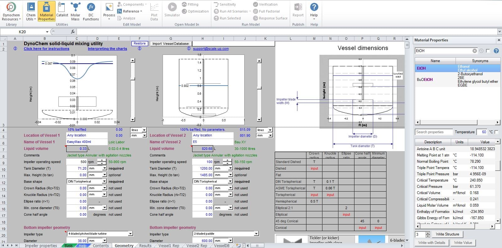
DynoChem Interface
DynoChem for Crystallization Development
The DynoChem Scale-up SuitTM provides a wide range of modelling tools and intuitive excel based utilities that are designed to help chemists and engineers overcome scale-up challenges. At CARBOGEN AMCIS, the use of modelling techniques by first intent is becoming more commonplace.
One such application is the translation of stirring speed from laboratory to production scale. The typical approach taken by CARBOGEN AMCIS during scale-up is to keep the energy input per unit mass constant (W/kg). Similarly, the same approach can be used to scale-down, for instance; if laboratory scale experiments must be used to trouble-shoot unexpected problems in production.
Case study: Scale-down and the counterintuitive behaviour of a crystallization-process
Very occasionally, processes, with a robust track record can lead, e.g. prior to the process validation, to an unpredictable out-come. This is typically linked to parameters which are usually not obvious. If this is the case, then small changes can sometimes have major consequences.
In 2019, a long-running process at CARBOGEN AMCIS began to exhibit unpredictable behaviour during the final crystallization. A crust formation was identified as a possible reason for the low yield and purity of some batches. As a result, the crystallization team at the Neuland site were asked to investigate.
We began our investigation by experimentally determining the metastable zone width (MSZW) of the final crystallization. It quickly became apparent that the point of seeding was very close to the point of maximum oversaturation. 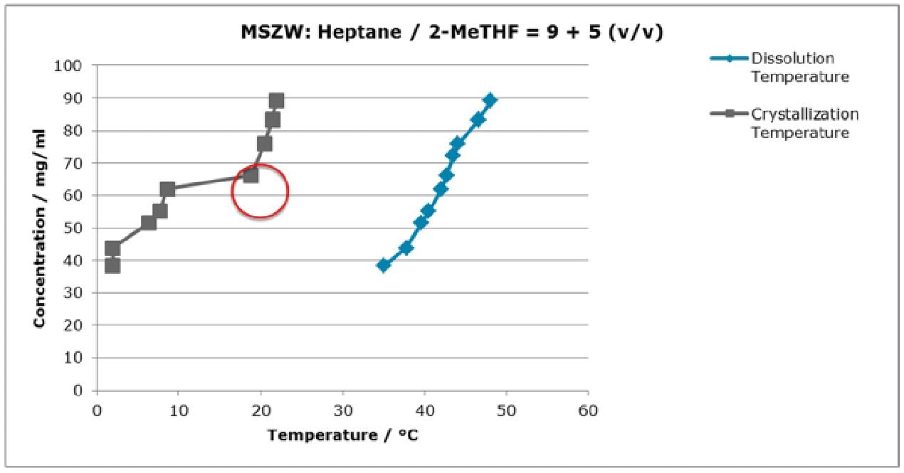 Table 1: Meta-stable zone determination
For further work the solvent system was adjusted to a lower degree of supersaturation by altering the ratio between solvent (Methyl-THF) and anti-solvent (Heptane).Despite this reduction of the supersaturation, the crust formation reoccurred several times during the lab investigation. Worthy of notice was that none of the conducted experiments showed reproducible results.
We next decided to look into the stirrer speed. In order to improve our process understanding without additional experimentation, DynoChem was used to translate the stirrer speed of our laboratory experiments into the equivalent stirrer speeds on scale-up and vice versa.
The model employed keeps the power input per unit mass constant. The results are listed from low to high energy.
 Table 2: Actual (highlighted in blue) and modelled stirrer speeds. *Ran in Duplicate
The data reveals that the crystallization requires a minimum amount of energy to prevent crust formation. It also shows that the difference between 73 and 100 rpm was crucial for the manufacturing. The batches at 199 and 216 rpm were conducted after the investigation and showed repeatability of the process refinements (stirring speed set to > 150 rpm).
The formation of the crust was directly linked to liquid-liquid-demixing (i.e. oiling out). The higher turbulent shear rate helped to avoid droplet formation and the energy input seemed to trigger amorphous contents to be re-dissolved.
This is a good example of how DynoChem can lead to the results which are not directly accessible by classical process development. DynoChem provided the visualisation tools and models needed to quickly and easily understand this counterintuitive behaviour of the investigated crystallization system.
Case Study: Comparison of two continuous flow reactors to demonstrate equivalency for the purpose for PAR studies
Here at CARBOGEN AMCIS we are developing high throughput continuous flow processes to greatly improve and simplify what would otherwise be complex or hazardous batch reactions. The efficient heat and mass transfer characteristics of flow reactors makes them ideal for highly exothermic reactions or for reactions involving highly reactive or unstable intermediates.
Typically, there are fewer challenges associated with scaling-up flow processes – The simplest way is to extend the duration of the continuous run to process more material; however, increasing the length or diameter of the reactor may be necessary to achieve the step-change in throughput that is desired. Changing the reactors dimensions impacts several parameters unique to flow systems, such as; axial dispersion, mixing efficiency and heat transfer, all of which can be modelled using DynoChem tools and utilities.
In one such a scenario at CARBOGEN AMCIS we have needed to characterise the mixing parameters of a laboratory scale reactor (RLab) and a production scale reactor (RProd). The throughput of RProd is approximately 5x that of RLab; therefore, performing PAR experiments using RProd is not practicable due to the quantities of starting material required. The objective of this work has been to identify the conditions at which the two reactors demonstrate mixing equivalency to provide a solid justification of performing PAR work in RLab irrespective of flow rate and throughput.
Through application of the DynoChem tools, in combination with other literature precedent, we have been able to accurately model the mixing time (tmixing,Kenics) as a function of flow rate, as described using equation (1).
Equation (1): tmixing, Kenics = ai Re-nKenics
Where:
tmixing,Kenics is the mixing time specific to the Kenics type static mixers used in both RLab and RProd.
ai is the mixing parameter which is a combination of constants derived from; reactor
dimensions, mixer type and the kinematic viscosity of the reaction solution.
Re is the Reynold’s number dependent on reactor dimensions and which changes as a function of flow rate.
nKenics is the exponent constant describing the rate of change of mixing as a function of flow rate.

Graph 1: Flow rate vs. mixing time with determined values for exponent nKenics and fitting parameter ai.
To obtain the graphical linearity flow rate and mixing time are plotted on a double logarithmic scale.
By fitting experimental data to the model we are able to determine the mixing parameter and exponent constants specific to RLab and RProd in both laminar and turbulent flow regimes and identify the transition point between the two regimes.
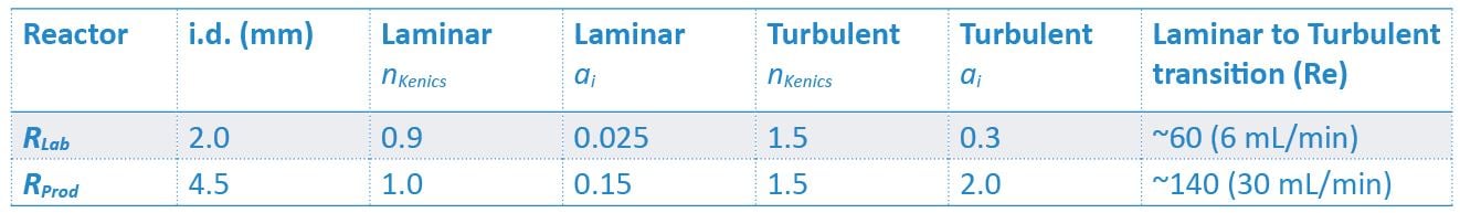 Table 1: Experimentally determined constants for laboratory and production reactors
With the model complete it is possible to determine the flow rates in RLab and RProd at which an equivalent degree of mixing is obtained.
The next task is to obtain some conversion data as a function of flow rate from a simple kinetic experiment using RLab. By increasing the flow rate from 20 to 100 mL/min at intervals of 20 mL/min two sets of analysis were performed on samples that were immediately quenched on exiting the flow reactor and on samples that were allowed a prolonged post-flow stir-out period before being quenched.

Graph 2: Effect of flow rate on conversion (left axis). Re, tRes and tMixing are also plotted on a logarithmic scale (right axis) for comparison.
The first key observation is that extending the stir-out period after the reaction has exited the flow reactor effectively decouples the effect of flow rate on residence time and hence conversion reaches a maximum above 40 mL/min. The second key observation is that conversion drops off by 1-2% from 40 mL/min to 20 mL/min, therefore; we can conclude that 40 mL/min is the minimum flow rate required to achieve a desirable conversion. (Some repeat experiments are required to confirm this cut off point).
Using the model that has been generated the mixing time and the flow rates at which RLab and RProd are equivalent can be determined.

Table 2: Minimum flow rate and Re at which RLab and RProd demonstrate equivalent tMixing with no detrimental effect on reaction conversion
According to the model, an experiment carried out in RLab at > 40 mL/min will proved the same result as the same experiment carried out in RProd at > 320 mL/min.
As it is the intention to run RLab at 60 mL/min and RProd is typically running at 400 mL/min with the intention to increase throughput to 950 mL/min, this work confirms that any PAR or DoE work completed in RLab will be valid for RProd above the defined flow rates.
The use of modelling techniques, with the help of the DynoChem Scale-up SuitTM, by first intent for scaling continuous flow reactor systems and understanding reaction kinetics in such systems will ensure the continued development of safe and robust continuous chemistries at CARBOGEN AMCIS.
Part (1/2)